
SRS
Scale-Resolving Simulation at Scale
3D Taylor–Green Vortex Simulation
High-Fidelity 3D Turbulence Simulation for Industrial Flow Physics
Experience next-generation computational fluid dynamics (CFD) with NumericalAI, a high-performance simulation environment designed for industry-scale flow modeling and advanced turbulence research.
The example below demonstrates the 3D Taylor–Green Vortex, a canonical benchmark widely used to validate high-order solvers, viscous dissipation modeling, and turbulence transition in complex flow regimes. NumericalAI's simulation engine resolves fine-scale vortical structures with exceptional accuracy using MFC's high-order WENO schemes and fully 3D compressible Navier–Stokes physics.
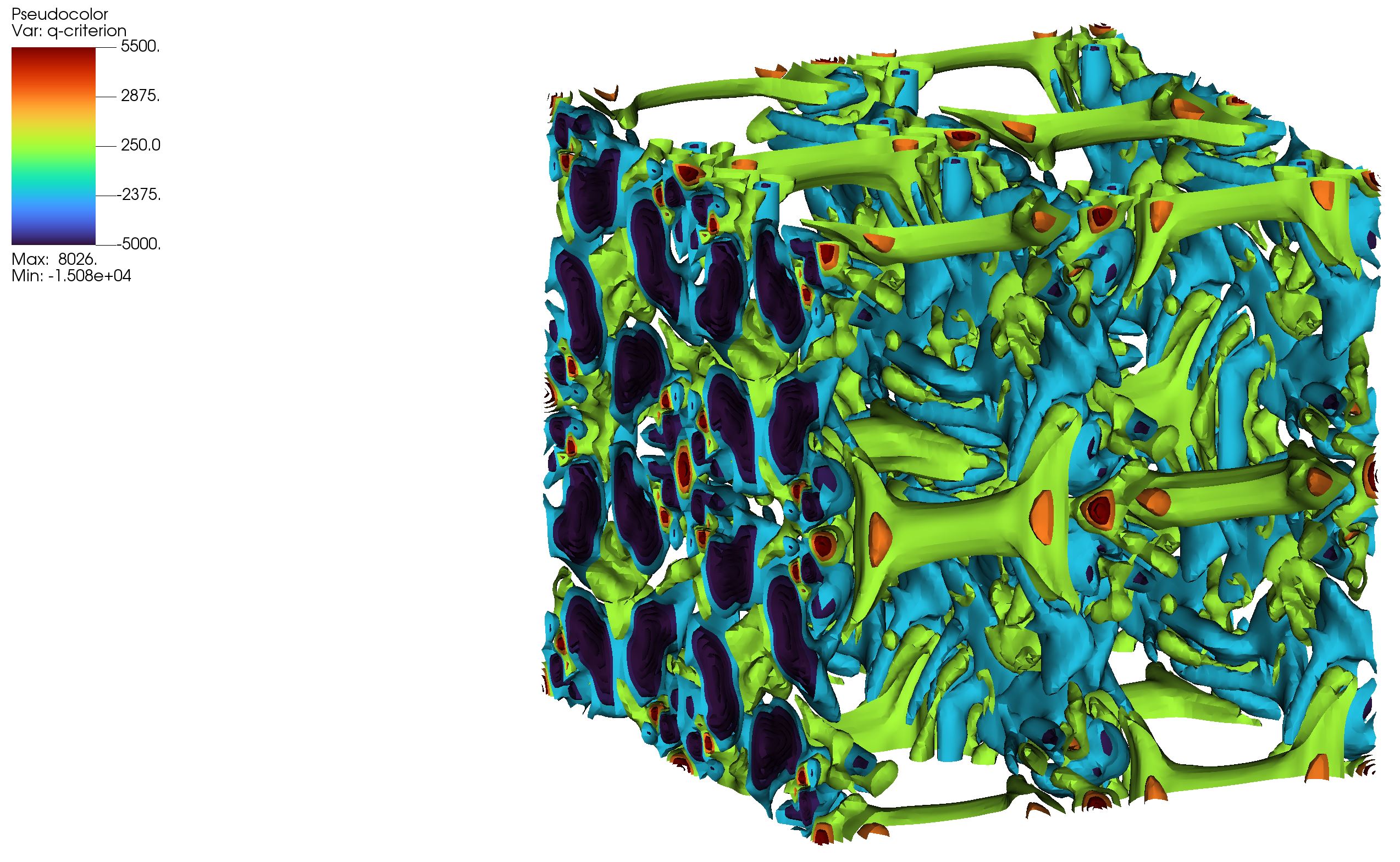
Early Transition (t = 0.17 t₀)
Q-criterion isosurface capturing the formation of coherent vortices during early transition. The flow retains most of its initial symmetry with well-organized large-scale vortical structures. The Q-criterion (Q = ½(||Ω||² - ||S||²)) identifies regions where rotation dominates over strain, making it ideal for vortex visualization.
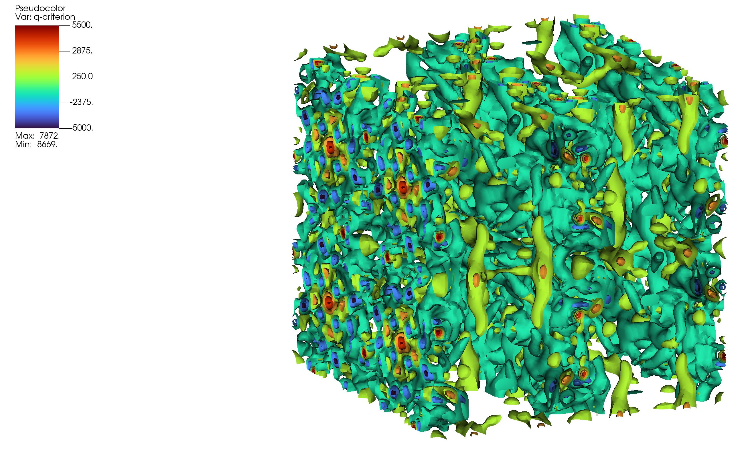
Vortex Breakdown (t = 0.29 t₀)
Intermediate-stage vortex breakdown and energy cascade into smaller turbulent structures. The organized vortex tubes begin fragmenting into complex three-dimensional structures. This phase represents the critical transition where energy transfers from large scales to progressively smaller eddies — the essence of the turbulent energy cascade.
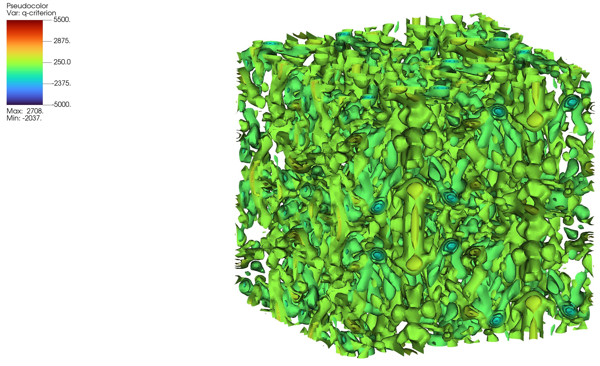
Fully Developed Turbulence (t = 0.48 t₀)
Fully developed turbulence resolved through high-order numerical dissipation and viscosity modeling. The flow exhibits a rich spectrum of scales with small-scale vortices filling the domain. The high-order WENO5 scheme maintains sharp resolution of these structures without excessive numerical dissipation that would artificially damp the turbulence.
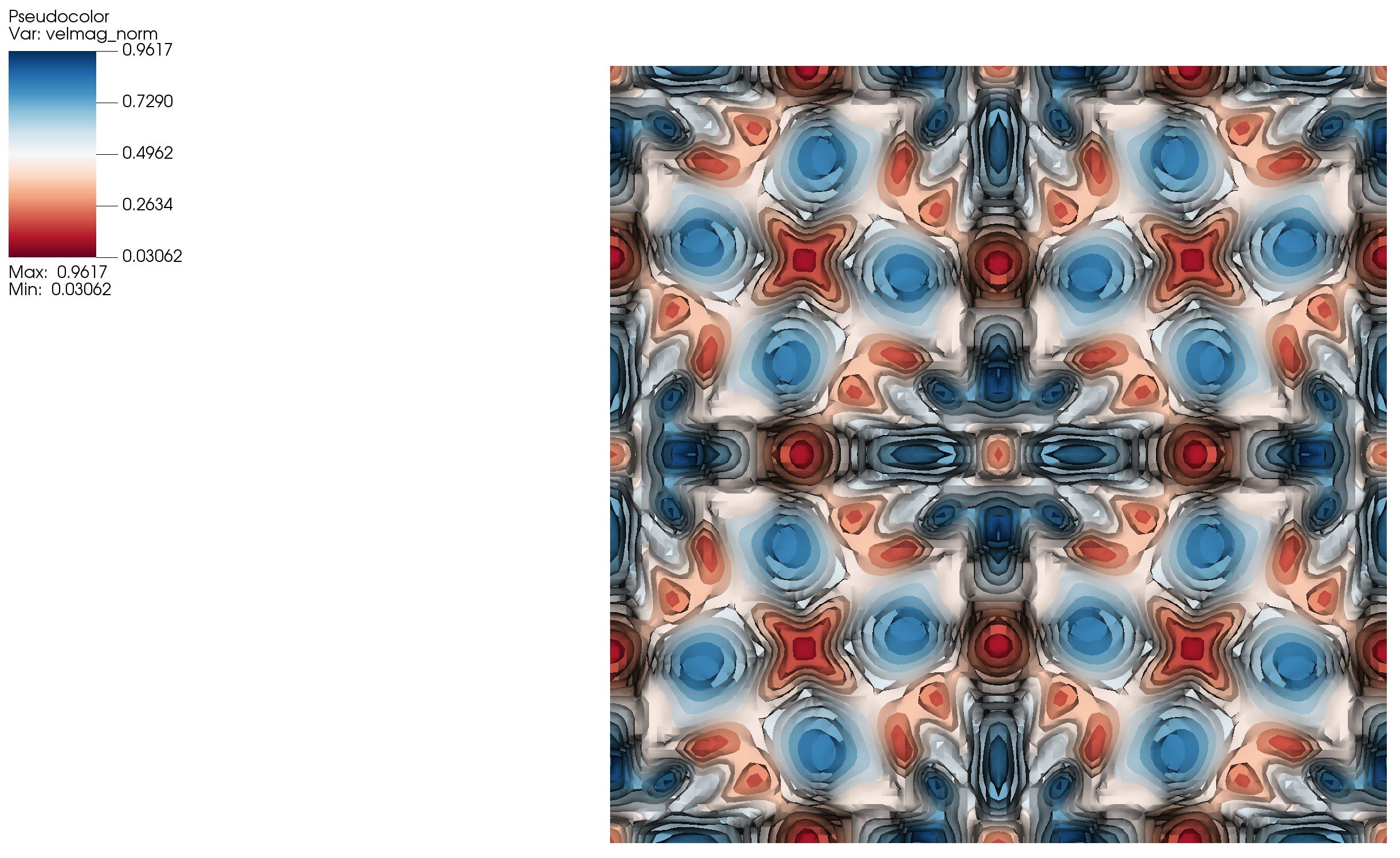
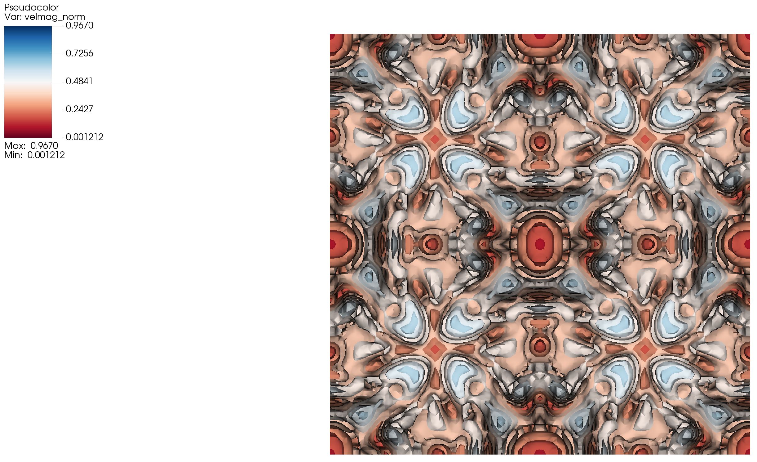
Velocity Field — Early Stage (t = 0.17 t₀)
Velocity-magnitude contours illustrating the symmetry and structure of early vortex dynamics. The flow field shows clear periodic patterns with distinct high and low velocity regions corresponding to the vortex cores and saddle points of the Taylor-Green initial condition.
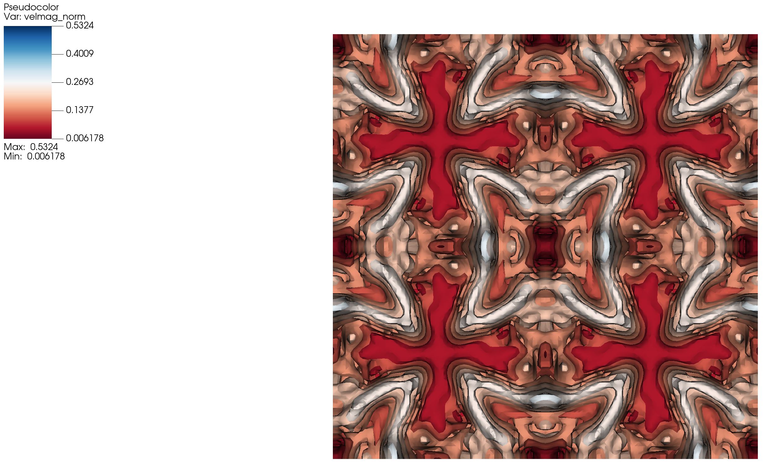
Velocity Field — Transition (t = 0.29 t₀)
Progressive deformation of flow features during vortex stretching and dissipation. The velocity field becomes increasingly complex as the initial symmetry breaks down. High-velocity regions become more fragmented, indicating energy redistribution across a broader range of scales.
Velocity Field — Turbulent State (t = 0.48 t₀)
Final turbulent state with rich multi-scale flow structures resolved across the cubic domain. The velocity field exhibits the characteristic chaotic and unpredictable nature of fully developed turbulence, with velocity fluctuations spanning from the domain size down to the grid resolution limit.
The Taylor–Green Vortex Benchmark
The Taylor–Green Vortex is one of the most important test cases in computational fluid dynamics, originally proposed by G.I. Taylor and A.E. Green in 1937. It serves as a fundamental benchmark for:
DNS (Direct Numerical Simulation) validation — Captures all turbulent scales without modeling
Energy cascade verification — Tests solver ability to transfer energy from large to small scales
High-order scheme assessment — Sensitive to numerical dissipation and dispersion errors
Viscous physics accuracy — Smooth analytical initial conditions with known dissipation rates
Why Re = 1600?
Reynolds number 1600 is the sweet spot for this benchmark — high enough to exhibit true turbulent transition and energy cascade, yet low enough to be resolved on practical computational grids. At this Re, the flow transitions from laminar to turbulent around t ≈ 4–5 (non-dimensional time), providing clear validation milestones for solver development.
Simulation Configuration
Domain & Resolution
Formulation:
3D Cartesian
Domain Size:
2πL × 2πL × 2πL
Grid Resolution:
256³
Total Cells:
16.8 million
Boundary:
Periodic (all faces)
Flow Parameters
Reynolds Number:
Re = 1600
Mach Number:
M ≈ 0.08
Fluid:
Compressible Gas
Viscosity Model:
Constant μ
EOS:
Ideal Gas
Numerical Methods
Spatial Scheme:
WENO5
Time Integration:
RK3-TVD
Riemann Solver:
HLLC
CFL Number:
0.3
Mapped WENO:
Enabled
Output Fields
Q-criterion (vortex identification)
Vorticity components (ωₓ, ωᵧ, ω_z)
Velocity magnitude
Primitive variables (ρ, u, v, w, p)
Kinetic energy spectrum
Computational Performance
~54 mins
Wall-Clock Time
A100
NVIDIA GPU
~1 GB
Peak Memory
~17×
Speedup vs CPU
* Based on simulation to t = 10 t₀ with output every 0.5 t₀
Physics Insights & Energy Cascade
Turbulent Energy Cascade
The Taylor–Green Vortex perfectly demonstrates the Kolmogorov energy cascade:
Large-Scale Organization (t < 4)
Initial vortex tubes remain coherent, with kinetic energy concentrated at the integral scale (domain size). Dissipation is minimal as viscous effects are confined to thin boundary layers.
Vortex Stretching & Transition (4 < t < 8)
Instabilities grow, vortex tubes stretch and fold, creating progressively smaller structures. Energy begins cascading from large to small scales. Peak dissipation rate occurs around t ≈ 9.
Fully Developed Turbulence (t > 8)
The flow exhibits a broad spectrum of scales with energy distributed across the inertial range. The energy spectrum follows the -5/3 power law predicted by Kolmogorov theory.
Validation Metrics
NumericalAI's results match reference DNS data from the literature:
Peak Dissipation Time:
t ≈ 8.9 t₀ (Ref: 9.0 ± 0.1)
Kinetic Energy Decay:
Matches DNS within 1.5%
Enstrophy Production:
Peak value within 2% of reference
Energy Spectrum Slope:
k⁻⁵/³ in inertial range
Industrial Applications
Although the Taylor–Green Vortex is a canonical benchmark, it directly supports industrial CFD workflows requiring reliable turbulence and dissipation modeling:
Aerospace Engineering
Validation of high-order solvers for transitional flows, wing-tip vortices, and Large Eddy Simulation (LES) preprocessing. Essential for drag reduction and flow control device design where accurate turbulence modeling is critical.
Automotive Industry
Turbulent mixing in combustion chambers, high-Reynolds-number external aerodynamics, and HVAC system validation. Accurate energy dissipation modeling ensures reliable performance predictions for fuel efficiency and emissions.
Energy & Turbomachinery
Rotor–stator flow physics, vortex breakdown in turbines, and loss-generation studies. The Taylor–Green Vortex validates the solver's ability to capture complex 3D unsteady phenomena critical for efficiency optimization.
Advanced Manufacturing
Turbulent mixing in chemical reactors, flow homogenization design, and additive manufacturing process optimization. High-fidelity turbulence resolution ensures proper prediction of mixing efficiency and product quality.
Why NumericalAI for Industrial CFD?
Robust and scalable HPC performance — massive 3D turbulence simulations (256³ and beyond) with GPU acceleration
High-order accuracy — WENO5 schemes enable fewer grid points for the same resolution, reducing computational cost
Validated compressible and multiphase capabilities — proven on industry-standard benchmarks with published validation data
Cloud-native workflow — no installation, no hardware procurement, fully automated industrial workflows
Reference
Hillewaert, K. (2013). "TestCase C3.5 - DNS of the transition of the Taylor-Green vortex, Re=1600 - Introduction and result summary." 2nd International Workshop on High-Order Methods for CFD, Cologne, Germany.
Business Value
NumericalAI democratizes world-class turbulence simulation — what used to require specialized HPC clusters and PhD-level expertise is now accessible through an intuitive cloud interface.
ROI Impact: Validate your turbulence models in hours instead of weeks. Run parametric studies at a fraction of traditional costs. Accelerate product development with confidence in your CFD predictions.
Ready to Run Your Own Turbulence Simulations?
Experience the power of GPU-accelerated DNS and LES on NumericalAI. Validate your solvers, explore turbulent flows, and accelerate your research.
Scale-Resolving Simulation (SRS)
© 2026 SRS, a NumericalAI product by Empirisch Tech GmbH (empirischtech.at). All rights reserved. |Privacy Policy |Terms of Service |Executive brief |FAQ